Introductory Tutorial¶

In this first contact with the SimCX framework, we will walk you through its basic components and create an example project in that process.

The framework has been mainly developed as a tool to teach complex systems. As such, a lot of the design decisions are biased towards that purpose. Most of the examples have also that bias.

In SimCX there are three base components (implemented as python classes): The Simulator that implements the simulation core, the Visual that is used to show the state of a simulator, and the Display that controls one application window and can contain several visuals. We then provide, in two submodules, several specific implementations of simulators and visuals. You can use these, or create your own simulators and visuals, by deriving the base classes. Regarding the visual components, the framework supports the use of matplotlib (through the MplVisual class), or you can use OpenGL directly using the pyglet module.

The framework is generic in the sense that we can use several modelling and simulation paradigms, like difference equations, differential equations, or agent-based modelling. In this first tutorial we will focus on using difference equations to simulate a dynamical system.

Installation¶

Before we start, we need to install SimCX and all its dependencies. Be aware that the framework has been developed for Python 3, and mainly tested on that version. Nevertheless, we make an effort to make it compatible with Python 2.7.

SimCX is available from the PyPI repository. To install, on a terminal (Command Prompt on Windows), execute the following command:

$ pip install simcx

That command will install SimCX and all its dependencies. Make sure that the pip command you are running is from the Python version you wish to install the framework on. On Windows, the pip command may not be on the system path. In that case you will need to provide the full path to the pip executable, or navigate to its directory before executing.

Model Description¶

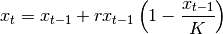
In this tutorial we will use SimCX to model population growth using difference equations. We will use an example taken from Hiroki Sayama’s book Introduction to the Modeling and Analysis of Complex Systems [1]. To start we will model a population with exponential growth, using the following equation:

$x_t = a x_{t-1}$

Here, $x_t$ is the population size at time step $t$ , $x_{t-1}$ is the population size at time step $t-1$ , and $a$ is the growth ratio of the population per time step. This simple model will give us an unbounded exponential growth of the population, which is not very life like. We can thus consider adding a bound to the size of the population, using the following equation:

$x_t = x_{t-1} + r x_{t-1} \left(1 - \frac{x_{t-1}}{K} \right)$

We have introduced a new parameter $K$ that represents the carrying capacity of the environment. Also, we have made the following substitution $r=a-1$ . To get more details on the mathematical modelling and derivation of these equations, refer to [1].

Implementing the Model¶

Let us start with the implementation. We will first need to import the SimCX package. We will also need some of the ready-made simulator and visual classes from the sub-modules. In this example, we will use the simulators.FunctionIterator simulator and the visuals.TimeSeries visual.

import simcx
from simcx.simulators import FunctionIterator
from simcx.visuals import TimeSeries

We now need to define the function for our first difference equation. To accommodate different values for our growth rate parameter, we define a python function that in turn returns a function.

def eq1(a):
    return lambda x: a * x

Next we will create a new window to control our simulation. This is done by creating a new instance of the Display class. By default the window is created with a size of 500x500 pixels. You can change this using the width and height parameters of the constructor. We will also need our simulator and a plot to analyse the behaviour of our system. In this case we will use a time series plot.

display = simcx.Display()

a = 1.2     # The growth rate
x0 = 10     # The initial population size
sim = FunctionIterator(eq1(a), x0)

orbit = TimeSeries(sim)

display.add_simulator(sim)
display.add_visual(orbit)

simcx.run()

The code is self-explanatory. We first create the display, then we set the values for our parameters, and create the simulator. We then create the visual, and add both to the display. We now have everything setup to run our simulation, and to do that, simply call the function run(). This function will enter the main loop of the program, displaying the window and awaiting user interaction. The default keyboard bindings are:

Space: Continue or Pause simulation
S: Step the simulation
R: Reset the simulation (if the simulator supports it)
ALT+R: Start recording the window
F: Show or hide frames per second

By default, when a display is created, it is in paused mode. You can then run the simulation step by step by using the S key, or let the simulation run with the Space key. After some iterations of the simulation, you should se something like what is shown in Fig. 1.

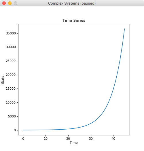
Fig. 1 Time series plot of the first model.

It is clear that the population has an exponential growth, and if you try to continue running the model, you will see that it just keeps increasing. Let us then improve our simulation, by using the second equation where we introduce the environments carrying capacity. We will need to define a new function.

def eq2(r, K):
    return lambda x: x + r*x*(1 - (x / K))

We now need to change our main code block to accommodate this new equation.

display = simcx.Display()

a = 1.2
x0 = 10
K = 1000
sim = FunctionIterator(eq2(a - 1, K), x0)

orbit = TimeSeries(sim)

display.add_simulator(sim)
display.add_visual(orbit)

simcx.run()

Again, running our simulation for some time, we should get something similar to what is shown in Fig. 2.

Fig. 2 Time series plot of the second model.

We now can see that our population does level out when approaching the carrying capacity of the environment. We can further analyse this system by testing different initial conditions. Fortunately, both the simulator and visual classes used, allow us to set more than one value for the initial state. By changing the line:

x0 = [0, 10, 200, 1000]

We are now testing all these four initial values for the population size. Run the simulation and see what you get.

To end this first tutorial we will make a movie of our simulation run. The framework already provides this capability. To create the movie, you can simply add to your code, before the simcx.run() line, the following:

display.start_recording('movie.mp4')

This will create a movie file, with the filename provided. The recording will span the whole simulation run. From the start, up to the application close. For each step of the simulation, one frame will be recorded. By default, the movie will be recorded with a frame rate of 20 fps, but that can be changed by passing the fps parameter to the Display.start_recording() method. We can also alter the bitrate of the recording from the default of 1800 Kbps. You can also start a recording during any simulation without adding any code, simply by using the ALT+R keyboard shortcut. In that case, the file will have the default name of simcx.mp4.

In this example we mostly made use of the simulators and visuals that are provided with the framework. To make full use of SimCX, though, you may need to implement your own simulators and visuals. To get an idea of how the ones used in this tutorial work, have a look at the reference (and code) for both the simulators.FunctionIterator and the visuals.TimeSeries classes. In another tutorial we will show you how to create your own.